Explainable Artificial Intelligence (XAI)
Artificial Intelligence (AI) has been used in several fields to solve various problems, including Natural Language Processing, Image classification, and segmentation. It increases the attention of the other scientific communities. Convolutional neural networks (CNNs) show excellent potential in adapting models defined for natural images to other image domains. However, Learning-based methods have the disadvantage of not being completely clear about their logic, so their confidence may be in doubt.
On this website, you will find a set of tools that allow you to interpret some of the characteristics of your CNN models.
Interpretability vs Explainability
Interpretability or transparency denotes the characteristic of a model that makes sense to a human observer. At the same time, explainability refers to any action or procedure performed by a model to clarify or detail its internal functions.
We enumerate some of the reasons that show the necessity of interpreting the decision process of AI methods:
- Trust the model. Relevant, e.g., Medical doctors and final users.
- Fairness. Relevant, e.g., patients and individuals affected by model decisions.
- Possibility to improve models and adapt methods to a new field. Relevant, e.g., researchers, data scientists, and developers.
- Identify and remove bias in the training dataset.
- Correct adversarial perturbations that could alter a prediction.
Categorizing based on locality
Local methods
The explainability of the model is reduced to the interpretation of the prediction of specific input samples. A common approach is to feed a model with known input (i.e., image) and observe the model's behavior for the expected class (see what part of the input is more relevant).
Global methods
It can explain how a model works without testing a specific set of inputs. For instance, in a linear classifier, the weights can show the level of importance that the model assigns to every attribute. An outweigh feature can alter the confidence of the classification.
XAI Apps
Interactive Tool for Visualizing CNN Predictions
Interactive tool allows users to visualize the connection between changes in peak intensity and prediction outcomes within the CNN framework. The tool enables the selection of an input spectrum and a target class to modify the model logit. By applying a delta change to significant peaks identified using XAI-2DCOS, users can observe changes in the model's output and how the spectrum shifts within the feature space. This visualization helps understand how boosting confidence for one class by adjusting the logit could simultaneously increase the logit for another class, potentially shifting the spectrum closer to the domain of another class.
- We can select between different classes: Oil classes, delta and Sample number.
The tool displays the probabilities, logit values, and predicted classes before and after the adjustments. This approach provides a practical example of the intricate balances and risks associated with CNNs, highlighting the potential for unintentional shifts across class boundaries. Through this visualization, users gain a deeper understanding of how changes in peak intensity can influence model outcomes and the complex interactions within the feature space.
Sample number changes according to the selected Oil classes, it means, lower the Sample number higher the model response.
Fourier Domain Analysis
Convolutional neural networks (CNNs) convolve input functions such as images, signals,
ands text with kernels in the spatial domain.
A CNN can be expressed in the Fourier domain.
The components of the network can be analyzed in this domain, which allows us to broaden its interpretation.
The convolution theorem expresses that the Fourier transform of a convolution of two functions is
the pointwise product of their Fourier transforms.
Convolution theorem
Consider two functions \(g(x)\) and \(h(x)\) with Fourier transform \(G\) and \(H\), where \( \mathcal{F}\) denotes the Fourier transform and \( \mathcal{F}^{-1}\) is the inverse Fourier transform operators then: $$ r(x) = \{g*h\}(x) = \mathcal{F}^{-1}\{G\cdot H\}$$
Visual Representation of the Convolution theorem
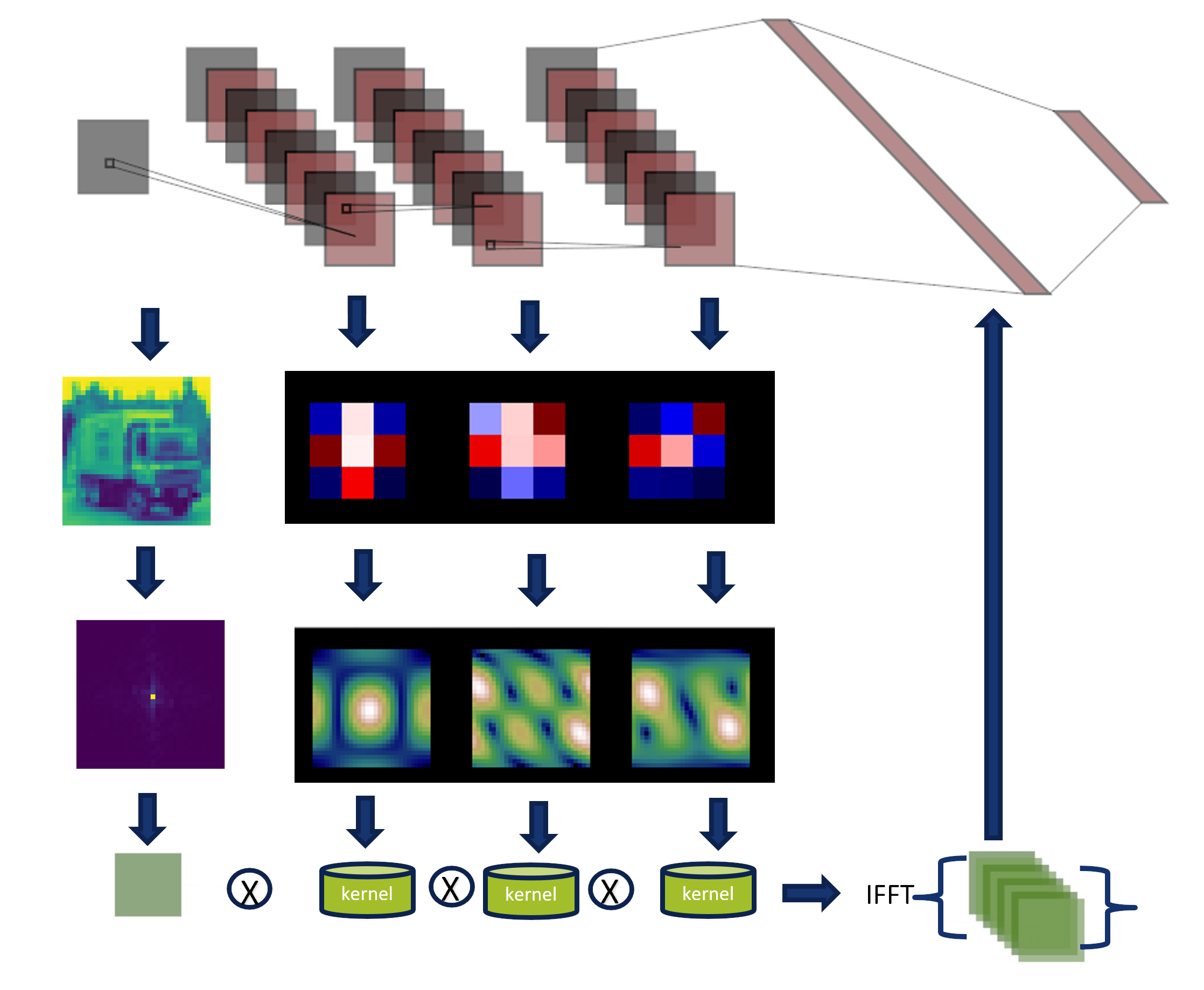
The convolution theorem express that convolutions in the spatial domain are
multiplication in the Fourier domain.
Similarly, the image shows us how the kernels and the input image are transformed in the Fourier domain.
They are multiplied, and the inverse transform is applied to generate a classification.
On this page, we show three approaches to transform a network defined and trained
in the spatial domain to the Fourier domain.
Shallow Network and Datasets
| Dataset | Input size |
Kernel size |
Firs layer Output size |
Kernel size |
Second layer Output size |
Kernel size |
Third layer Output size |
Dense layer Output ize |
Classes |
|---|---|---|---|---|---|---|---|---|---|
| MNIST (1 vs 7) | (28, 28, 1) | (1, 64) | (28, 28, 64) | (64, 64) | (28, 28, 64) | (64, 64) | (28, 28, 64) | (728, 64) | 2 |
| CIFAR 10 | (32, 32, 1) | (1, 64) | (32, 32, 64) | (64, 64) | (32, 32, 64) | (64, 64) | (32, 23, 64) | (1024, 64) | 10 |
| CIFAR 10 PAD | (42, 42, 1) | (1, 32) | (42, 42, 64) | (32, 64) | (42, 42, 64) | (64, 128) | (42, 42, 64) | (1762, 64) | 10 |
This shallow network comprises three convolutional layers followed by a dense and final classification layer.
The 2D Convolutions don't include activations, bias, or pooling.
In the Fourier analysis, we used two datasets, MNIST and CIFAR10.
MNIST dataset contains images for the numbers 0 to 9. However, we used a subset of numbers 1 vs. 7.
Additional to the standard version of the CIFAR 10 dataset, we included a version adding zero padding (5 pixels) around the border.
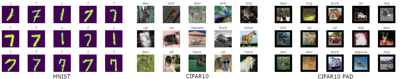
We do not publish metrics of the results because our interest lies in the visualization of the kernels. Below, we show a series of experiments performed using this simple CNN. However, later we will enable the possibility of including your models to be analyzed.
Fourier Network 1
This approach is possibly the slowest, most redundant,
nevertheless the most straightforward approach that provides many advantages
when implementing operations not directly defined in the Fourier space.
In this approach, first layer kernels and the input signal are transformed to the Fourier domain
and multiplied to produce an output.
The output is converted to the spatial domain to implement some actions like:
- Padding
- Pooling
- No Linear activations
- Batch normalization, etc.
Then, the result is transformed to the Fourier domain and used as input in the new layer.
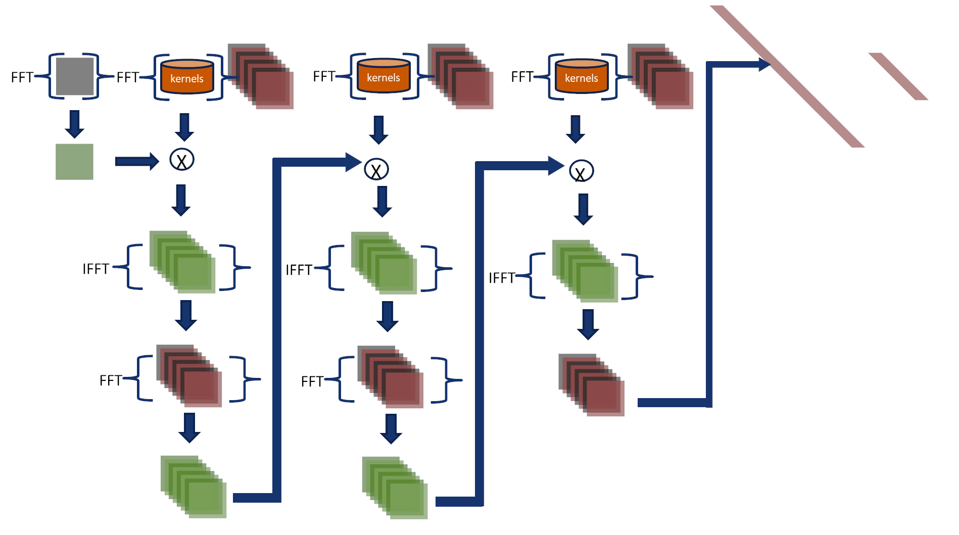
Fourier Network 2
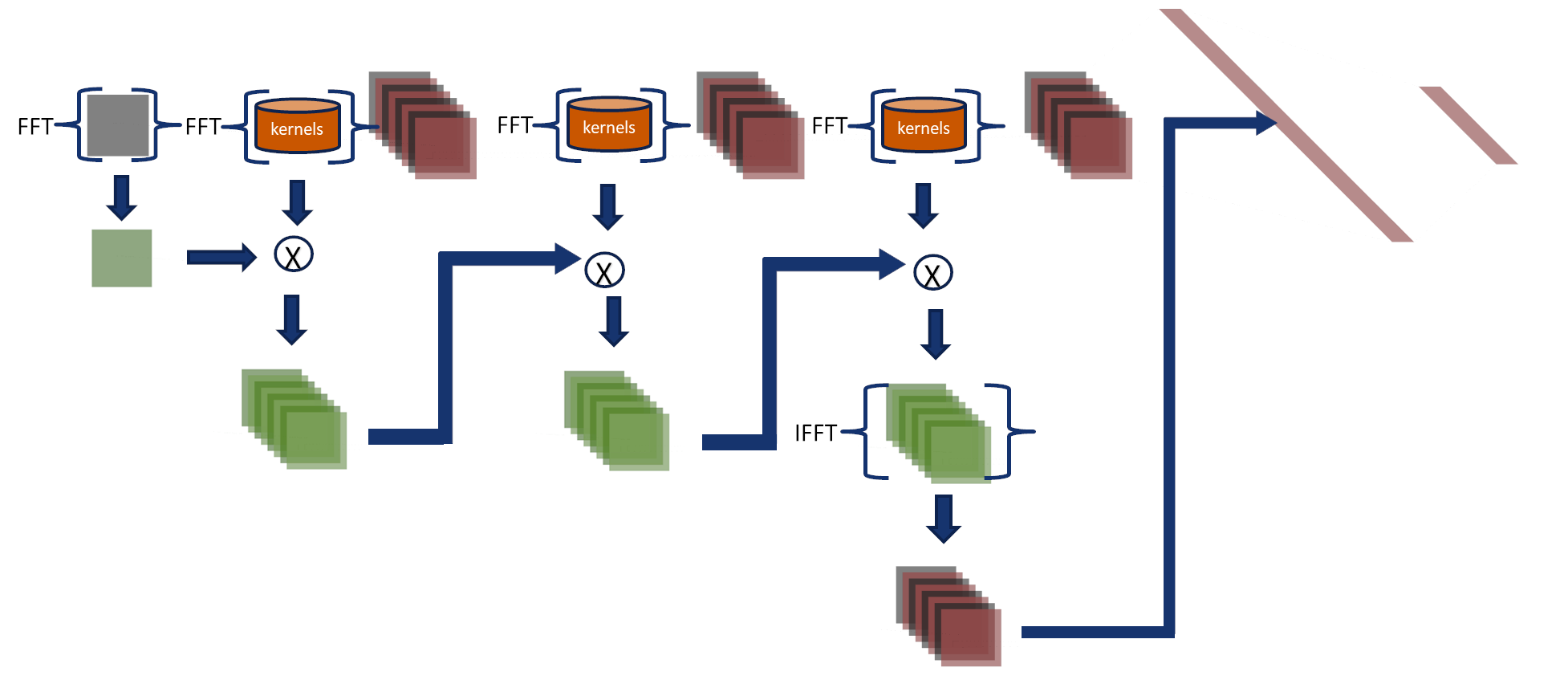
This approach does not transform intermediate results to the spatial domain,
making it faster than Fourier-Net 1.
In this approach, the convolutions are performed in the Fourier domain,
and their output feeds the final two layers.
- Kernels and input images are transformed to the Fourier domain and multiplied in a cascade (see the figure).
- The inverse Fourier transform converts the output, and then it is used to feed the fully connected layers in the spatial domain.
Accumulative error
CNNs add padding to images to compute features on the image borders and after each layer,
the padding is set to zero.
Fourier-Net 2 adds padding to input images and only removes it in the last step.
Therefore, it accumulates an error layer after layer around the image edges.
Fourier Network 3
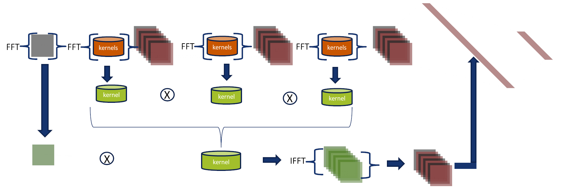
Fourier-Net 3 uses the associative property
Consider three functions \(f(x)\), \(g(x)\) and \(h(x)\) with Fourier transform \(F\), \(G\) and \(H\), where \( \mathcal{F}\) denotes the Fourier transform and \( \mathcal{F}^{-1}\) is the inverse Fourier transform operators then: $$ r(x) = \{f*g*h\}(x)= \mathcal{F}^{-1}\{(F\cdot G)\cdot H\} = \mathcal{F}^{-1}\{F\cdot (G\cdot H)\}$$ In this approach, the convolutions are performed in the Fourier domain, and their output feeds the final two layers.
- Kernels and input images are transformed to the Fourier domain.
- Using the associative property, we combine kernels from three layers into a single kernel in the Fourier domain.
- We multiply the input and the combined kernel.
- The inverse Fourier transform converts the output, and then it is used to feed the fully connected layers in the spatial domain.
Accumulative error
CNNs add padding to images to compute features on the image borders and after each layer,
the padding is set to zero.
Fourier-Net 3 adds padding to input images and only removes it in the last step.
Therefore, it accumulates an error layer after layer around the image edges.
The Chain Rule
Taylor-based* (TD) and Layer-wise Relevance Propagation** (LRP) methods
produce relevance maps that associate each pixel with a score indicating its contributions to the classification decision using partial derivatives of the model weights.
To compute the derivative of the input w.r.t. the input image,
we can divide our function (network) into two subfunctions to improve the analysis.
[*] G. Montavon, S. Lapuschkin, A. Binder, W. Samek, and K.-R. Müller, “Explaining nonlinear classification decisions with deep Taylor decomposition,” Pattern Recognit., vol. 65, pp. 211–222, May 2017, doi: 10.1016/j.patcog.2016.11.008.
[**] S. Bach, A. Binder, G. Montavon, F. Klauschen, K.-R. Müller, and W. Samek, “On Pixel-Wise Explanations for Non-Linear Classifier Decisions by Layer-Wise Relevance Propagation,” PLOS ONE, vol. 10, no. 7, p. e0130140, Jul. 2015, doi: 10.1371/journal.pone.0130140.
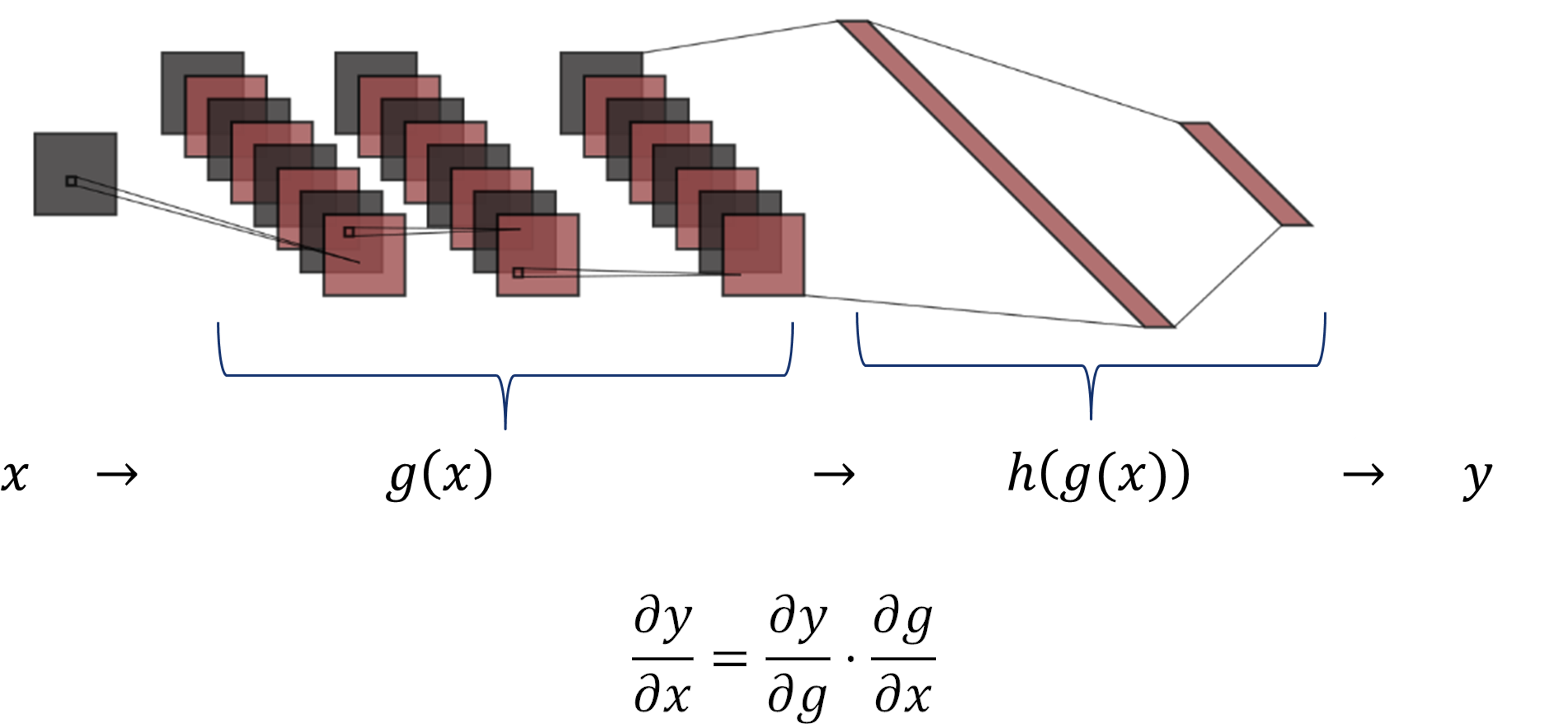
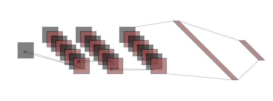
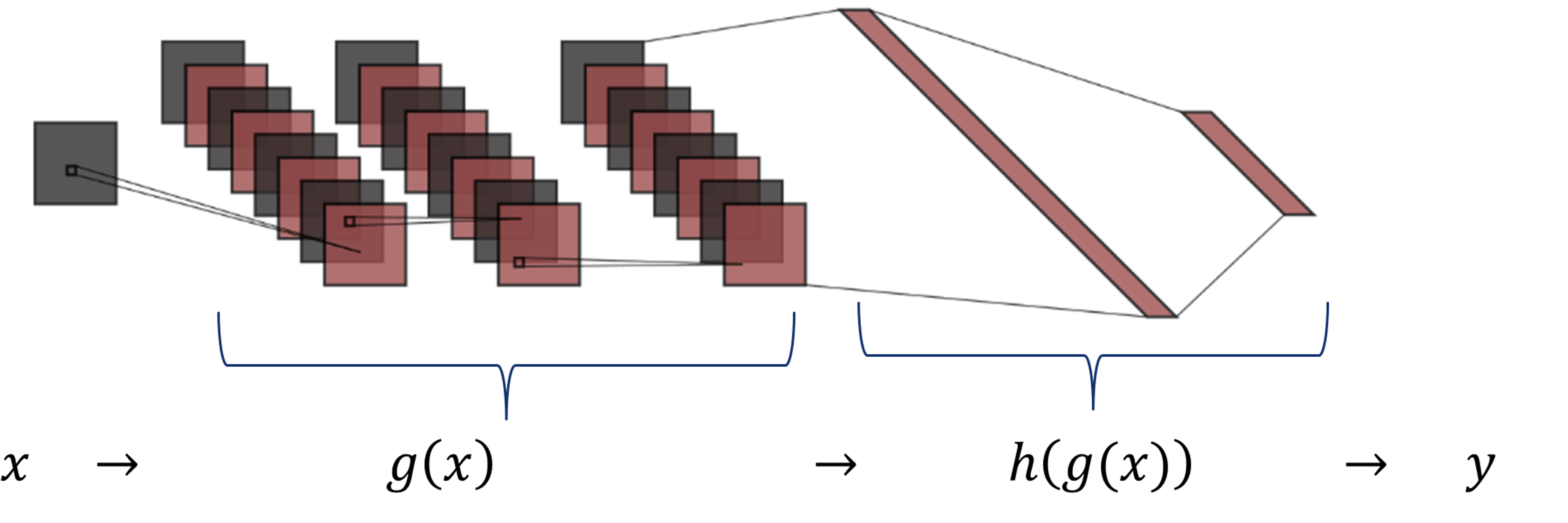
As shown in the figure, the function \(g(x)\) includes the three convolutional layers, and \(h(g(x))\) comprises the two dense layers.
The chain rule expresses the derivative of the composition of two differentiable functions \(g\) and \(h\) in terms of their derivatives.
For this network, it is possible, to compute the derivative of \(y\) w.r.t. the \(g(x)\) and then compute the derivative of \(g(x)\) w.r.t. the input image \(x\).
$$ \frac{\partial y}{\partial x} = \frac{\partial y}{\partial g} \cdot \frac{\partial g}{\partial x}$$
Example with 1D function
We define a simple function and compute gradients using Tensorflow, we first compute \(\frac{\partial y}{\partial x} \):
# x is the input
x = tf.Variable(3.0)
b = tf.Variable([3., 4.])

# compute gradients using Tensorflow
with tf.GradientTape() as tape:
    g = x * b
    y = tf.reduce_sum(g** + 5)

# tape.gradient computes the gradient of output (y) w.r.t input (x)
dy_dx = tape.gradient(y, x)

# print function outputs
print("g(x): ",   g.numpy())
print("h(g(x)):", y.numpy())
# print derivative
print("dy/dx :", dy_dx.numpy())
--------------------------------------------------------------------------
g(x):  [ 9. 12.]
h(g(x)): 307880.88
dy/dx : 513135.0
tape.gradient(output, input) computes the gradient of the output (\(y\)) w.r.t the input (\(x\)).
The chain rule slipts the function in two parts: \(\frac{\partial y}{\partial x} = \frac{\partial y}{\partial g} \cdot \frac{\partial g}{\partial x}\).
We compute first \(\frac{\partial y}{\partial g} \):
# x is the input
x = tf.Variable(3.0)
b = tf.Variable([3., 4.])

# compute gradients using Tensorflow
with tf.GradientTape() as tape:
    g = x * b
    y = tf.reduce_sum(g** + 5)

# tape.gradient computes the gradient of output (y) w.r.t intermediate value (g)
dy_dg = tape.gradient(y, g)
# print derivative y w.r.t g
print("dy/dg :",dy_dg.numpy())
--------------------------------------------------------------------------
dy/dg : [ 32805.004 103680.]
Now, we compute \( \frac{\partial g}{\partial x} \):
# x is the input
x = tf.Variable(3.0)
b = tf.Variable([3., 4.])
# compute gradients using Tensorflow
with tf.GradientTape() as tape:
    g = x * b
    y = tf.reduce_sum(h**+5)

# tape.jacobian computes the gradient of output (g) w.r.t input (x)
dg_dx = tape.jacobian(g, x).numpy()
print("dg/dx :", dg_dx)
--------------------------------------------------------------------------
dy_dg/dx : [3. 4.]
tape.jacobian(output, input) computes the jacobian of the output (\(y\)) w.r.t the input (\(x\)).
Finally, we apply the chain rule \( \frac{\partial y}{\partial x} = \frac{\partial y}{\partial g} \cdot \frac{\partial g}{\partial x} \)
# Apply chain rule
# dy/dx = dh/dx * dy/dh
dy_dx = np.sum(np.multiply(dy_dg, dg_dx))

print("dy/dx :", dy_dx)
--------------------------------------------------------------------------
dy/dx : 513135.0
As expected, the same result is obtained. The treatment for 2D images is similar but more complex.
We will take this advantage to focus our efforts on \(g(x)\) and use the Fourier properties to comprehend more about our network.
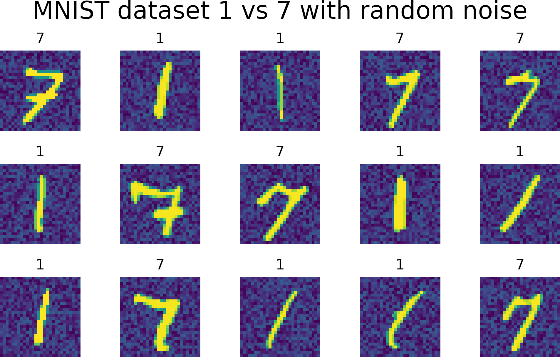
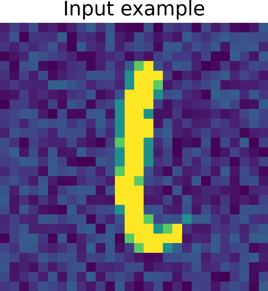
Experiments on MNIST dataset
MNIST dataset contains images for the numbers 0 to 9. However, we used a subset of numbers 1 vs. 7.
We added uniform noise 0 - 0.3 to the images.
Training len 13000, Testing len 2163 images.
Model description
We define a network with three convolutional layers and two dense layers, linear activation, and no Biases.
Code:
model = tf.keras.Sequential([
        keras.Input(shape=(28, 28, 1)),
        keras.layers.Conv2D(64, 3, padding="same", use_bias=False),
        keras.layers.Conv2D(64, 3, padding="same", use_bias=False),
        keras.layers.Conv2D(64, 3, padding="same", use_bias=False),
        keras.layers.Flatten(),
        keras.layers.Dense(256, activation='relu'),
        keras.layers.Dense(2, activation='softmax')
    ])
Model summary:
Model: "sequential"
_________________________________________________________________
    Layer (type)                Output Shape              Param #
=================================================================
    conv2d (Conv2D)             (None, 28, 28, 32)        288

    conv2d_1 (Conv2D)           (None, 28, 28, 64)        18432

    conv2d_2 (Conv2D)           (None, 28, 28, 128)       73728

    flatten (Flatten)           (None, 100352)            0

    dense (Dense)               (None, 256)               25690368

    dense_1 (Dense)             (None, 2)                 514

=================================================================
Total params: 25,783,330
Trainable params: 25,783,330
Non-trainable params: 0
Similar information can be found in the following table.
| Dataset | Input size |
Kernel size |
Firs layer Output size |
Kernel size |
Second layer Output size |
Kernel size |
Third layer Output size |
Dense layer Output ize |
Classes |
|---|---|---|---|---|---|---|---|---|---|
| MNIST (1 vs 7) | (28, 28, 1) | (1, 32) | (28, 28, 32) | (32, 64) | (28, 28, 64) | (64, 128) | (28, 28, 128) | (256) | 2 |
Training Histograms
We train with Adam optimizer, learning rate = 1e-4 and epochs = 100.
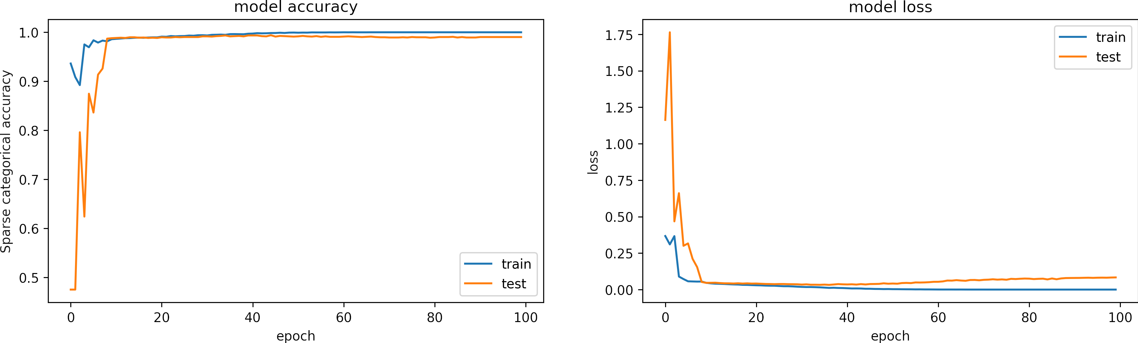
The following figure shows the training history for the accuracies and losses.
We observe that the model learns in less than 20 epochs.
The training accuracy is 1.00 and training loss 7e-6.
The testing accuracy is 0.999 and testing loss is 0.083.
CNN duality Spatial and Fourier domains
We express this CNN in the Fourier domain to analyze their components (Fourier-Net 3),
which allows us to broaden its interpretation.
Input and kernels are then transformed using the Fast Fourier Transform (FFT),
storing frequency and amplitude information.
They are multiplied, and the inverse Fourier transform is applied to convert the output back into the spatial domain to feed the fully connected layers.
Visualization of some kernels for the 1st , 2nd and 3rd layers

Fusion of the kernels of layers 1, 2 and 3
In the absence of activation functions, kernels of adjacent layers can be combined into more meaningful kernels employing the associative property.
We tested this property in our network, reducing it from 10272 to 128 kernels.
Fourier kernels are obtained by multiplying kernels of layers 1, 2, and 3.
The inverse Fourier transform can be applied to visualize kernels in the spatial domain with dimensions 7x7.
These kernels produce the same output as obtained for the original model.

Analisys of the convolutional block
As shown in the figure, the function \(g(x)\) includes the three convolutional layers, and \(h(g(x))\) comprises the two dense layers.
The Chain Rule allow us to slipts the gradients of our network in two parts:
\( \partial y/ \partial x = \partial y/ \partial g \cdot \partial g/ \partial x\).
In this example, we focous on the analysis of convolutional part \(\partial g/\partial x\).
Later, we find the derivatives in Fourier space and analyze their implications.
Derivative of convolution
The derivative of a convolution is the derivative of one of the functions convolved by the other function: $$ \frac{\partial}{\partial x}\Big( f1(x)*f2(x) \Big)= \left(\frac{\partial f1(x)}{\partial x}\right)*f2(x) = f1(x)*\left(\frac{\partial f2(x)}{\partial x}\right)$$ In our network, \(g(x)=x*K_{123}\) is the result of convolving the input signal \(x\) and the set of kernels \(K_{123}\). Therefore, the derivative of \(g(x)\) w.r.t. the input \(x\) is equal to: $$\frac{\partial g(x)}{\partial x} = \frac{\partial x}{\partial x}* K_{123}$$
Pixel-wise partials derivatives \(\frac{\partial x}{\partial x}\)
The input image \( x\) is a 2D array with dimensions \((n,m)\), in consecuence we calculate \((n\times m)\) partial derivatives of size \((n\times m)\).
Therefore, the matrix storing the partial derivatives has size \(((n\times m)\times (n\times m))\).
When calculating the partial derivative w.r.t at a particular pixel,
its derivate is equal to 1, and the other pixels are considered constant; therefore,
their derivative is zero, see figure.
Derivative of convolution in the Fourier Domain, \(\partial g/ \partial x\)
The Fourier transform of \( \partial g(x)/\partial x \) is the product of the Fourier transforms of \( \partial x /\partial x \) and \( K_{123}\) $$\mathcal{F}\left\{ \frac{\partial g(x)}{\partial x} \right\}= \mathcal{F}\left\{ \frac{\partial x}{\partial x}\right\} \cdot \mathcal{F}\left\{ K_{123}\right\}$$ The Fourier transform can be obtained using Python's Fast Fourier Transform (FFT) function. The following figures show the partial derivatives of the input image w.r.t. the pixels in the Fourier domain for both the real part and the absolute values.
| Real component \(\mathcal{F}\left\{ \frac{\partial x}{\partial x}\right\}\) | Absolute value \(\mathcal{F}\left\{ \frac{\partial x}{\partial x}\right\}\) | |
|---|---|---|
 |
 |
Finally, we multiply the previous result by the kernels to obtain the derivative of \(g(x)\) w.r.t. \(x\) in the Fourier domain \( \mathcal{F}\left\{ \frac{\partial g(x)}{\partial x} \right\}\),
the following figure shows some results:

Derivative of the output \(y\) w.r.t. \(g(x)\), \( \partial y/ \partial g\)
We compute the partial derivates of \( \partial y/ \partial g\) using the function tf.GradientTape() of Tensorflow (see Chain Rule).
First, we created a reduced model containing only \(h(g(x))\) and computed the gradients of \(y\) w.r.t. \(g(x) \)
Model: "Reduced model h(g(x))"
_________________________________________________________________
Layer (type)                Output Shape              Param #
=================================================================
input_1 (InputLayer)        [(None, 28, 28, 128)]     0

flatten (Flatten)           (None, 100352)            0

dense (Dense)               (None, 256)               25690368

dense_1 (Dense)             (None, 2)                 514

=================================================================
Total params: 25,690,882
Trainable params: 25,690,882
Non-trainable params: 0
The figure shows the partials derivate of the output \(y\) w.r.t. \(g(x)\), \( \partial y/ \partial g\) in the spatial domain. It has size \(28 \times 28 \times 128 \), which corresponds to the input size of this reduced model.
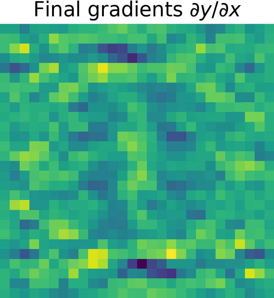
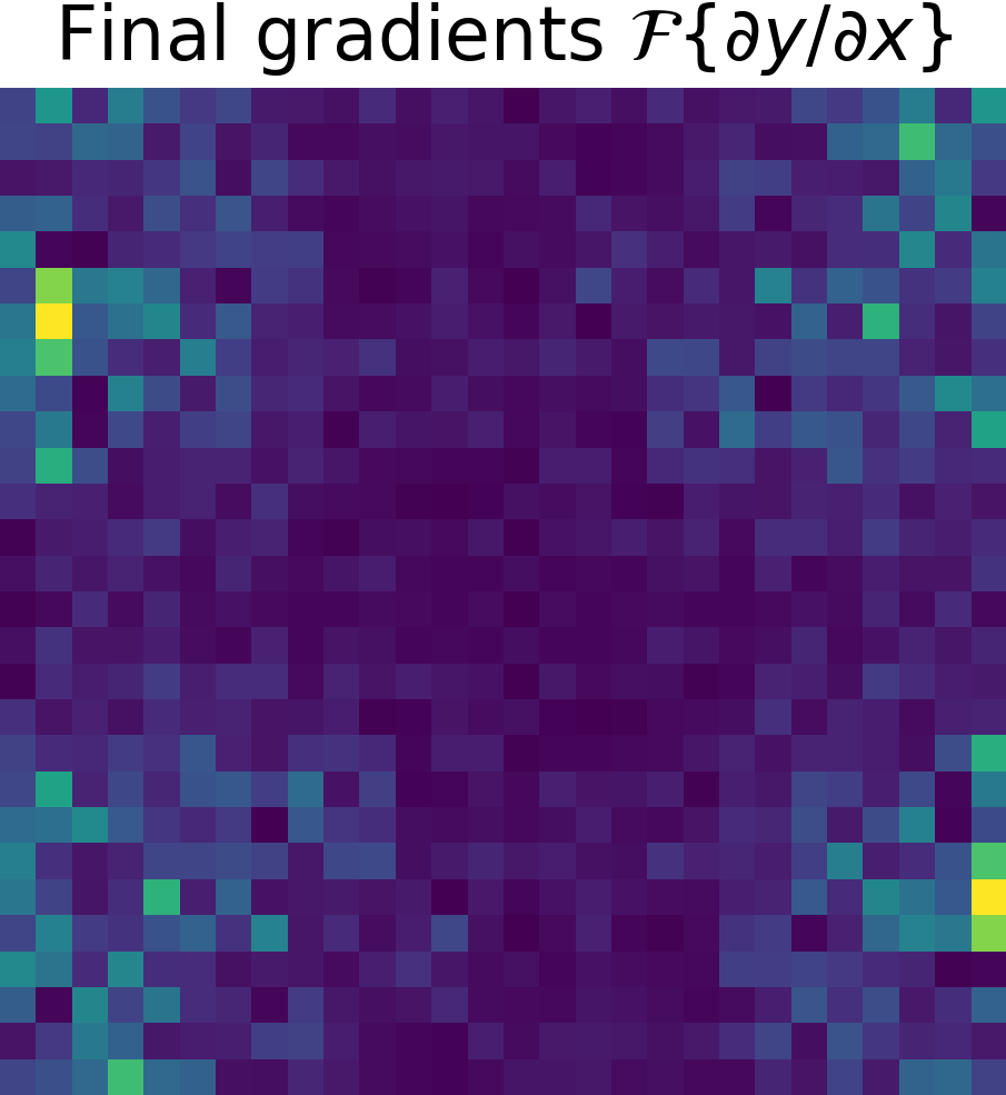
Derivative of the output \(y\) w.r.t. the input \(x\), \( \partial y/ \partial x\)
To finish, just apply the chain rule (see Chain Rule). $$ \frac{\partial y}{\partial x} = \frac{\partial y}{\partial g} \cdot \frac{\partial g}{\partial x}$$
| Final gradients \( \partial y/\partial x\) | Final gradients \(\mathcal{F}\left\{ \partial y/ \partial x \right\}\) | |
|---|---|---|
 |
 |
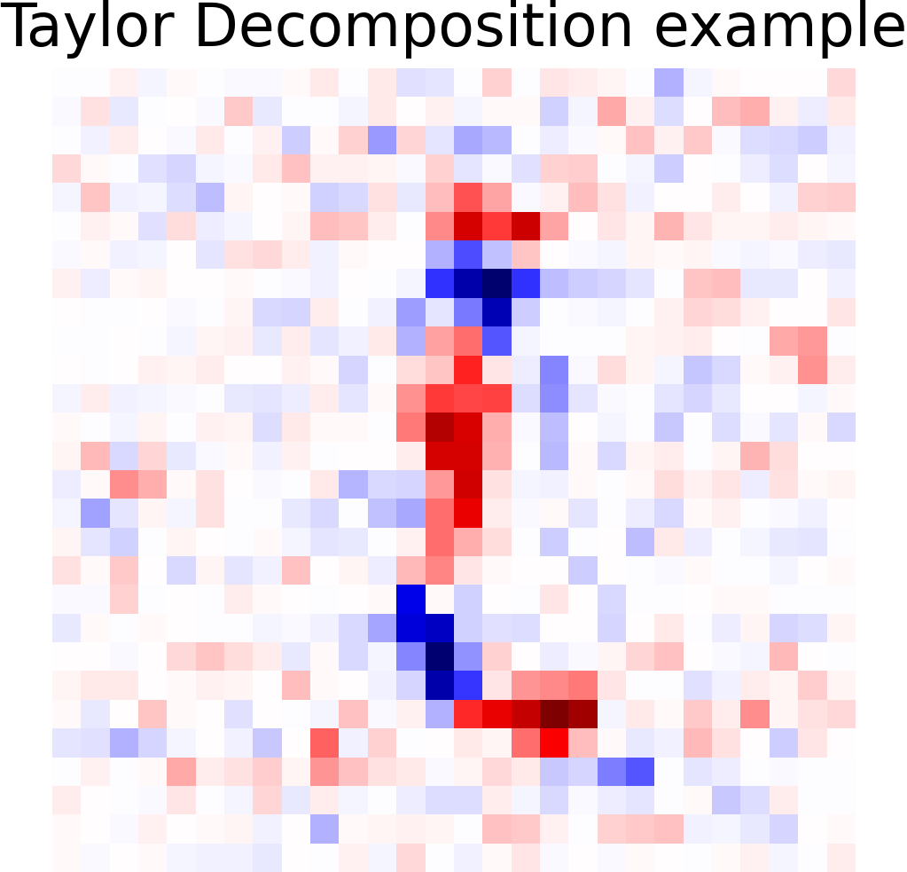
Taylor decomposition example
The first order Taylor expansion in the image space is defined as:
where:
- \(x \) is an input image
- \(\tilde{x}\) a root point
- \( \epsilon \) represents the higher order Taylor terms
\(R_p\) is the Relevance map that indicates which pixels are relevant for the prediction of a given class.
Observations:
- This method can be applied to any differentiable CNNs models.
- Need to find a meaningful root point \(\tilde{x}\) where to perform the decompostion.
In the following, we show the result of a Taylor decomposition to expose one of the possible uses of calculating the partial derivatives in the Fourier and spatial domains.
Later we will expand the information on the Taylor decomposition and show more applications of the partial derivatives of a model CNN.
| Input image\(x\) | Taylor decomposition = \( \partial y/\partial x *(x- \hat{x} ) \) | |
|---|---|---|
 |
 |
Combined Kernels Importance Analisys
Feature Selection
Feature selection is used to identify a subset of input variables to reduce the computational cost of modeling and improve model performance by removing redundant or unnecessary information. (i.e., Pearson's correlation coefficient, ANOVA correlation coefficient, Spearman's rank coefficient, and Kendall's rank coefficient).
Various approaches, including stochastic and statistical methods, evaluate the relationship between each input variable and the target variable and select the input variables that have the most substantial connection with the target variable.
These methods can be fast for 1D variables.
In our case, we do not desire to evaluate the global importance of the features but rather the importance of those features for our trained model.
Kernel Selection
We list below the steps to select a set of essential kernels.
- Consider two submodels as shown in the figure, \(g(x)\) includes the three convolutional layers, and \(h(g(x))\) comprises the two dense layers.
- \(g(x)\) output dimensions is \( (28,28,128)\), in total 128 output features.
- Transform \(g(x)\) in the Fourier domain.
- Using the associative property, combine kernels from three layers into a single kernel set of size \((1\times 128)\).
- For each image in the training dataset:
- Iteratively, set a channel to zero for all the 128 output channels.
- Multiply the input and the combined kernel (one channel is deactivated).
- Use the inverse Fourier transform to convert the output and feed \(h(g(x))\).
- Infer the logits and compare them with the entire model logits.
- Order the 128 predictions from worst to best result (a bad result indicates that the deactivated channel is relevant).
- Create an approximate model only with one activated channel (from the ordered list), then iteratively:
- Test the approximate model and compare it with the entire model.
- If the mean absolute error between the approximate logit and the full model logit is greater than 30% of the total value, include an additional channel to the model.
- Save a list of the necessary channels used to obtain an approximate model with an MAE of less than 30%.
- Create a histogram of the necessary channels (kernels) used in the approximate models. The histogram reveals which kernels are most required.
- The first part of this process can also be done stochastically.
| Histogram stores the required kernels for the training samples to creates an approximate model. | Interpret the pixel importance by observing the activations of the relevant kernels. | |
|---|---|---|
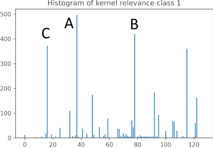 |
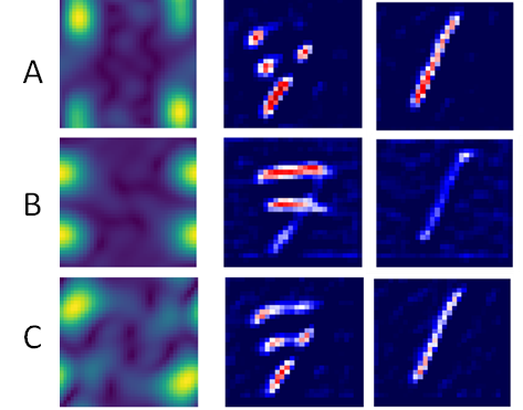 |
- We can see that kernel A activates the pixels that show vertical variation and that number 1 is fully activated while the rest of the image is not activated. The image of number 7 is partially deactivated.
- For kernel B, the image of number 1 is deactivated while the areas of the image of number 7 are activated where horizontal changes occur.
- In kernel C, the result is similar to kernel A, though the activation is smoother for number 1.
XAI Apps
Visualization App 1 (kernels)
This application shows sets of random kernels obtained by training a shallow network.
- We can select between three models: MNIST, CIFAR10 and CIFAR10PAD.
- The button Click here to generate new kernels randomly selects new sets of kernels for the given model.
Here we can observe random kernels obtained by training a shallow network with the dataset and their transformation in the Fourier space.
Visualization App 2 (kernels)
This application shows a kernel and the convolution output in the Spatial and Fourier domains.
- We can select between three models: MNIST, CIFAR10, and CIFAR10PAD
- The button Input randomly selects a new input image for the dataset.
- The buttons Layer 1, Layer 2, and Layer 3 randomly select a kernel of its respective layer.
- Drag and drop uploads an image to visualize its convolution in the Spatial and Fourier domains.
Visualization App 3 (Relevance Maps)
This application shows a Relevance map (R-map) that indicates which pixels are relevant for predicting a given class.
- This app takes the model and data presented in the LR-2D Example
- A posterior version will allow you to include your Tensorflow models.
- The first Dropdown selects a filter (Gaussian, Sharpness, or Nearest) used to create a perturbed input image.
- The slider Sigma selects the parameter of the respective filter.
- The slider Gamma controls the contrast of the output Relevance Map.
- The slider Image selects an image from a sample dataset with five classes (more information) .
- We can select between two options, when the model has Softmax activation: True, False
- We can select between two options to visualize numeric results: True, False (printed bellow the application).
Visualization App 4 (Model Summary)
This application shows the model summary.
It will soon show the model layers and their kernels in the Fourier and spatial domain.
Note: The Visualization at the moment is only possible for kernels of size 3x3.
The app allows you to select a specific layer and kernel.
The figure shows the input image and its convolution with the selected kernel.
However, note that the output of the channel depends on the input of the layer.
The figure also shows an image that is the average value of the channel input and the convolution result for that specific layer and kernel.
- The button Summary show a list of the layers operation.
- The button Summary conv show a list of the convolutional layers.
- The button Summary dense show a list of the dense layers.
- The button Summary others show a list of the other layers (i.e., BatchNormalization, ReLU, ZeroPadding2D, Dropout, GlobalMaxPooling2D, among others).
- The button Clear clear the screen
- The slider Layer Select the convolutional layer you want to visualize.
- The slider Kernel Select the kernel in the layer you want to visualize.
- The slider Image selects an image from a sample dataset with five classes (more information) .
Convolutional Neural Networks (CNNs) on Tensorflow
This section seeks to resolve some frequent questions and avoid possible errors in CNN programming in Tensorflow.
Here you will see fractions of code, the complete code can be found in a GitLab repository
(Python Course).
It contains series of Jupyter notebooks that will help you understand the basics of python and Tensorflow.
The examples given do not only seek to solve a specific problem.
Many exercises are written so that the concepts can be generalized.
Tensorflow hyperparameter selection
Learning Rate
During training, the network updates the learnable weights (\( w \)) depending on the error (\( Loss \)), which is the difference between the current prediction and the true value.
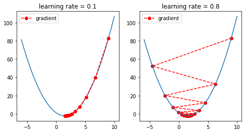
The learning rate (\( Lr \)) controls the gradient update.
$$ {w \leftarrow w - Lr \cdot \frac{\partial Loss }{\partial {w}}} $$
The learning rate rules the amount of change. Thus it is essential to select an adequate value.
Note: The definition of "small" or "large" depends on several factors, including the input scale.
For instance, a "large" learning rate for normalized images from 0 to 1 is definitely smaller than a "large" learning rate for an image with values between 0 and 255.
Similarly, a "large" learning rate (0.1) for a Raman spectrum with arbitrary units is larger than a "large"
learning rate (0.001) for normalized Raman spectrum because the intensity of normalized data is hundreds of times smaller.
There are four cases when selecting a learning rate:
- Too small: may result in a long training process that could get stuck, or may reach the maximum iteration before reaching the optimal point.
- Too large: may learn a sub-optimal set of weights or an unstable training process, it may not converge to the optimal point (jump around) or even diverge completely.
- OK: not very slow, not unstable. It is a commonly good solution, though it may not reach an optimal value.
- Learning rate scheduler: the learning rate is first large to accelerates initial training, then reduced in size as the number of epochs increases to help the network to converge.
Model performance
Classification metrics evaluate a model's quality. They provide valuable information.
However, it is essential to select an adequate metric.
We will briefly describe some concepts.
Confusion Matrix
A confusion matrix summarizes the performance of a classification outcome. The number of correct and incorrect predictions are summarized with count value into a matrix, it contains: True Positives (TP), True Negatives (TN), False Positives (FP), and False Negatives (FN).
| Predicted Positive | Predicted Negative | |
|---|---|---|
| Actual Positive | TP | FN |
| Actual Negative | FP | TN |
In the following, we create two confusion matrices for a binary classification problem in two cases and apply different metrics later.
Case 1. Balance data
The model predicted 120 samples as positive (C1) and 60 as negative (C2).
There were actually 80 C1 and 100 C2.
| Predicted Positive | Predicted Negative | Total | |
|---|---|---|---|
| Actual Positive | 70 (TP) | 10 (FN) | 80 |
| Actual Negative | 50 (FP) | 50 (TN) | 100 |
| Total | 120 | 60 | 180 |
Case 2. Inbalance data
The model predicted 3 samples as positive (C1) and 997 as negative (C2).
There were actually 10 C1 and 990 C2.
| Predicted Positive | Predicted Negative | Total | |
|---|---|---|---|
| Actual Positive | 1 (TP) | 9 (FN) | 10 |
| Actual Negative | 2 (FP) | 988 (TN) | 990 |
| Total | 3 | 997 | 1000 |
Accuracy
The term accuracy is often used to describe a good model performance. However, computer science has a specific definition of this term.
The accuracy score meassures the times a model classifies the samples correctly.
The accuracy can be defined using the confusion matrix:
Accuracy = (True Positives + True Negatives ) / All the Observations
Accuracy Case 1 = (70+50)/180 = 0.666
Accuracy Case 2 = (1+988)/1000 = 0.989.
The result looks fantastic, but the model fails to classify the positive prediction 9 of 10 times.
Therefore this metric is not showing the reality.
Balance Accuracy
Some literature defines the balanced accuracy using Sensitivity and Specificity, also known as the true positive and negative rates.
Balanced accuracy accounts for positive and negative outcome classes and is used with imbalanced data.
The accuracy can be defined using the confusion matrix:
Balanced Accuracy = (Sensitivity + Specificity) / 2
where,
Sensitivity = TP/(TP+FN)
Specificity = TN/(TN+FP)
Balance Accuracy Case 1 = (70/(70+10) + 50/(50+50))/2 = 0.6875
Balance Accuracy Case 2 = (1/(1+9) + 988/(988+2))/2 = 0.544
We can see that the Balance Accuracy for Case 2 is lower than using Accuracy, reflecting a result closer to reality.
For this reason, we recommend using different accuracy metrics for unbalanced data.
However, we define the balance accuracy as the average of sensitivity obtained on each class, where the best value is 1 and the worst value is 0.
Learning rate selection 1D Example
The Jupyter notebook can be found here .
Download and load Raman spectra data
You can download data from:
Bocklitz-Lab. Example-Raman-spectral-analysis. https://github.com/Bocklitz-Lab/Example-Raman-spectral-analysis. 2021. GitHub
The file DATA_dp_wc_bc.csv contains Raman spectra from mice tissues, averaged from each Raman map after despiking, wavenumber calibration and baseline correction.
The ID, annotation, and type of the tissues are included as separate columns in the file.
Load Data:
df = pd.read_csv("data/DATA_dp_wc_bc.csv")
Divide the dataset into training and testing.
It usually happens that a data set contains multiple samples from a single organism,
which could lead to errors and the concept of testing with training.
Therefore, to avoid bias, samples from the same mouse must be in the same subset either CV or T_V_T.
- T_V_T: training , validation, testing sets.
- CV: cross-validation with training and testing folds.
- Samples from the same subset start with a similar name, i.e., M10
- We select the first component of the name and transform them into a categorical class to split the dataset.
Code
# insert in postion 2 new column containing only the string before the first "_"
df.insert(2, 'name_split', df['Name'].str.split('_').str[:1].str.join(""))

# insert in postion 3 new column transfoming name_split to categorical
df.insert(3, 'name_split_cat', df['name_split'].astype('category').cat.codes)

# Find number of independet mice
number_samples = np.max(df['name_split_cat'])

print("number of independent samples : %d" %number_samples)

# print a section of the dataset, name_split_cat show the mouse index
print(df.iloc[15:25, 1:4])
Result
number of independent samples : 143

    Name      name_split  name_split_cat
M10_R1_I_007     M10            0
M10_R1_I_007     M10            0
M10_R1_I_008     M10            0
M10_R1_I_008     M10            0
M10_R1_II_001    M10            0
M101_B2_I_001   M101            1
M106_B2_II_001  M106            2
M11_C2_I_001     M11            3
M11_C2_I_002     M11            3
M11_C2_I_003     M11            3
We can observe some data examples. The samples from mice M10, M101, M106, and M11 have now a categorical names 0, 1, 2, and 3 respectively.
It will be used later to split the dataset on the mouse level.
T_V_T
A dataset can be divide into training, testing and validation.
In this example we randomly select training (70%), validation (15%) and testing (15%)
Code
# Shuffle mice index, as example we do not shuffle to visualize the result
# idx = np.random.permutation(np.arange(number_samples))
idx = np.arange(number_samples)

# select first 70% data for training
train_index = idx[:int(number_samples*.7)]

# select last 30% data to split into validation and test
temporal_index = idx[int(number_samples*.7):]

# select 15% data for validation
validation_index = temporal_index[:int(number_samples*.15)]
# select 15% data for testing
test_index = temporal_index[int(number_samples*.15):]

print("train idex : ", train_index)
print("validation idext : ", validation_index)
print("test index : ", test_index)
Result
train idex :  [ 0  1  2  3  4  5  6  7  8  9 10 11 12 13 14 15 16 17 18 19 20 21 22 23 24 25 26 27 28 29 30 31 32 33 34 35 36 37 38 39 40 41 42 43 44 45 46 47 48 49 50 51 52 53 54 55 56 57 58 59 60 61 62 63 64 65 66 67 68 69 70 71 72 73 74 75 76 77 78 79 80 81 82 83 84 85 86 87 88 89 90 91 92 93 94 95 96 97 98 99]
validation idext :  [ 100 101 102 103 104 105 106 107 108 109 110 111 112 113 114 115 116 117 118 119 120]
test index :  [ 121 122 123 124 125 126 127 128 129 130 131 132 133 134 135 136 137 138 139 140 141 142]
K-fold Cross validation
We can use sklearn to select the index to train and test K different models on different data folds.
In this example, we use five splits.
Note:
- A new model must be generated for each fold. Retraining a single model should be avoided.
- Auxiliar functions must be defined outside the cross-validation for the loop.
- In the following, we compute using the last fold's `train_index` and `test_index` to find the learning rate that best suit the model.
- We run cross-validation later.
Code
# import sklearn module
from sklearn.model_selection import KFold

# functions definitions to train a model here!

# define X as an array containing all mice index (0-142)
X = np.arange(number_samples)

# select the number of folds
kf = KFold(n_splits=5, shuffle=True)

# generate the splits
kf.get_n_splits(X)

# get the index for each split
for fold, (train_index, test_index) in enumerate(kf.split(X)):

    # model definition here!
    # model.fit here!

    # print index for testing, the index for training are the remainder
    print("Fold ", fold ," - Test index:", test_index)
Result
Fold  0  - Test index: [  1  17  33  36  38  39  56  62  64  67  81  82  83  86  88  95  97  98 100 105 106 111 113 119 120 122 124 129 136]
Fold  1  - Test index: [  5  12  15  16  20  21  22  31  32  34  37  41  45  51  57  59  61  63  69  73  89  91  93  94 115 128 134 137 138]
Fold  2  - Test index: [  8   9  11  14  24  26  27  49  50  60  65  74  76  78  79  87  92 101 102 103 104 108 109 114 117 126 130 139 140]
Fold  3  - Test index: [  0   3   4   7  13  19  35  42  46  47  53  54  55  58  68  72  75  85 99 107 110 112 121 123 125 127 141 142]
Fold  4  - Test index: [  2   6  10  18  23  25  28  29  30  40  43  44  48  52  66  70  71  77 80  84  90  96 116 118 131 132 133 135]
Examine the distribution of the classes
We can examine the distribution of the classes of the training subset by ploting the histogram over the classes.
Code
df[['class']].hist(figsize = (10, 5))
plt.title("Distribution of the classes")
plt.xticks(np.arange(4), classes)
plt.show()
Result
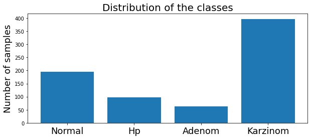
The dataset has four classes : Normal, HP, Adenom and Karzinom.
It is unbalanced. Nevertheless, it is not a critical situation, and we can continue.
Split dataset using the fold index
Prepare data to train:
Tensorflow requieres X and Y sets.
X (array): samples x dimension, we need to remove extra columns.
Y (array): samples x label.
Code
# list the dataset keys (column names)
keys_df = list(df.keys())

# elements to remove
remove_elements = ["Unnamed: 0", "Name", 'Annotation', 'Tissue', 'name_split', 'name_split_cat', 'class']

# remove keys from dataset keys list
for element in remove_elements:
    keys_df.remove(element)

# divide data into train and validation
Y_train = df.loc[df["name_split_cat"].isin(train_index), "class"]
X_train = df.loc[df["name_split_cat"].isin(train_index), keys_df]

Y_validate = df.loc[df["name_split_cat"].isin(test_index), "class"]
X_validate = df.loc[df["name_split_cat"].isin(test_index), keys_df]

# transform data into numpy arrays, cast Y to numpy int 32 dytpe
Y_train = np.array(Y_train, dtype=np.int32)
X_train = np.array(X_train)

Y_validate = np.array(Y_validate, dtype=np.int32)
X_validate = np.array(X_validate)
Normalization methods
We define three normalization methods.
- Normalize spectra by the norm.
- Standard normal variate.
- Normalize spectra by the integral between a range of wavenumbers .
def vector_normalization(v):
    # normalize spectra by the L2-norm
    norm = np.linalg.norm(v)
    if norm == 0:
        return v
    return v / norm


def snv(v):
    # SNV: Standard normal variate
    if  np.std(v) ==0:
        return v
    return (v - np.mean(v))/ np.std(v)


def normalize_integrated(v, wavenumber, wavenumber_min=1630, wavenumber_max=1690):
    # normalize spectra by the integral between the interval Wavenumbers/cm^{-1} wavenumber_min-wavenumber_max
    valid_Wavenumber = np.multiply(np.array(wavenumber)>=wavenumber_min, np.array(wavenumber)<=wavenumber_max).astype(float)
    integral = np.sum(valid_Wavenumber*v)

    if integral == 0:
        return v
    return v / integra
We plot the original Raman spectra and three normalization methods:

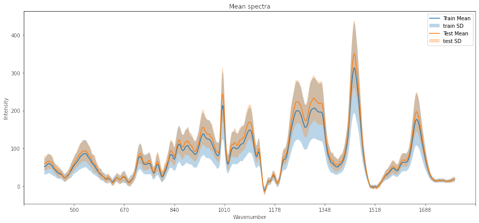
Ploting training and testing data
We can generate a plot of the mean and standard deviation of the training and testing dataset to observe similarities. The code for the plot can be found in the Jupyter notebook here .
Model definition
We define a simple model, the input has a shape of 691 Raman numbers, and the output has four neurons corresponding to the number of classes. We include three convolutional layers with bias and activations and two dense layers.
model = tf.keras.Sequential([
keras.Input(shape=(696, 1)),
keras.layers.Conv1D(32, 5, padding="same", use_bias=True, activation='relu'),
keras.layers.Conv1D(64, 5, padding="same", use_bias=True, activation='relu'),
keras.layers.Conv1D(128, 5, padding="same", use_bias=True, activation='relu'),
keras.layers.Flatten(),
keras.layers.Dense(256, activation='relu'),
keras.layers.Dense(4, activation='softmax')])
Neither the network configuration nor the final classification is our primary interest in this practice. Our goal is to recognize when the learning rate is adequate or not.
Define a number of epochs
There is no rule to define the number of necessary epochs. Some conditions require more epochs:
- CNN with several layers to train.
- A small learning rate.
- A large dataset.
We can start with a lengthy number of epochs epochs = 1000 to see how the training parameters respond (loss and accuracy).
Learning rate too large, learning_rate = 0.01
What can we observe on the plots?
- The training Accuracy (TA) value is set to 0 before the first iteration. After the first epoch, TA has a value of 0.52. This value is obtained after randomly initializing the kernels. That value is not relevant.
- Balance Accuracy shows a wide variation between two values, 0.5 and 0.7. However, the behavior of the model is better described with the loss and the accuracy.
- The accuracies and loses maintain invariable values. Thus, the model does not learn.
- The learning rate is too high that it can not converge.
- When the learning rate is very low, the same phenomena are observed.
Learning rate large, learning_rate = 0.001
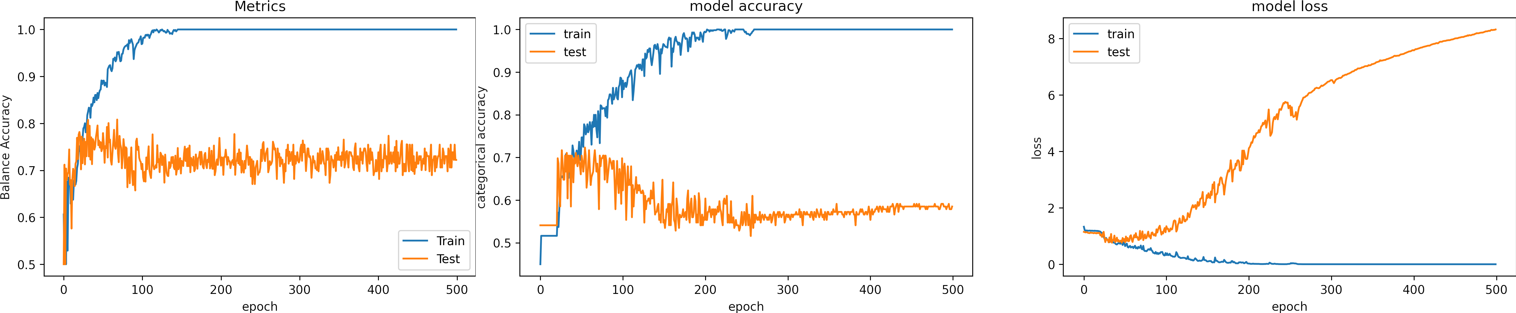
What can we observe on the plots?
- The model reach high training accuracy and low loss (1e-5) after 300 epochs.
- Around 300 epochs, the model reaches 100% accuracy, and the loss is too small and reduces over time. The model ceases to find a general solution, fits excessively to the input data (overfitting), and becomes more restrictive. .
- Overfitting is the most common reason why the loss for testing increases.
- The learning rate is high, it produces large fluctations in the training accuracy in the first epochs.
- It is possible to fall into local minima, and the model can get stuck with a high learning rate.
- Sometimes, the optimizer gets an good solution, but it jupms.
- The validation loss increases indicating overfitting.
- There was no need to train 500 epochs. Indeed it is better to stop the training earlier.
- In the case of cross-validation, it is recommended to test a fold to select the number of epochs.
- The results for testing are:
loss: 9.013
Accuracy: 0.572
Balance Accuracy: 0.365
Learning rate too small, learning_rate = 1e-6

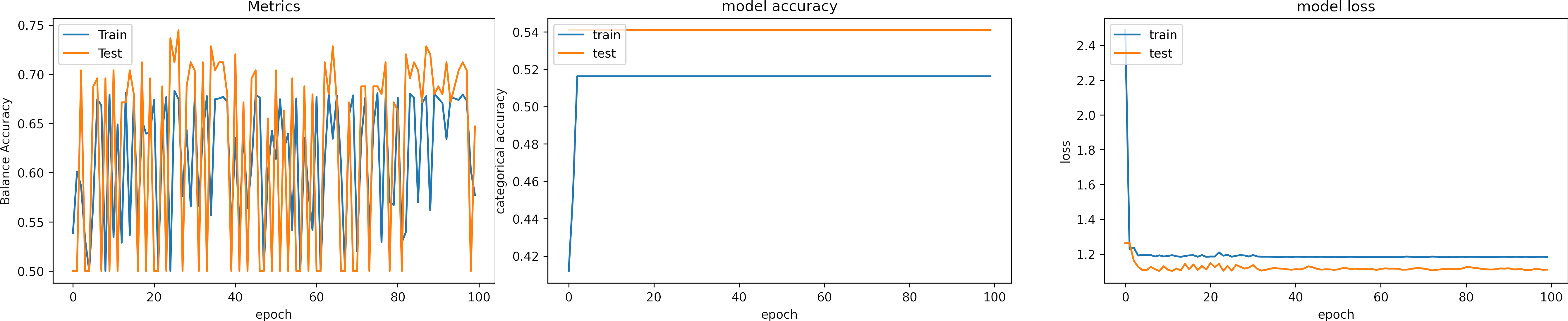
What can we observe on the plots?
- The training accuracy (TA) value is set to 0 before the first iteration. After the first epoch, TA has a value of 0.52. This value is obtained after randomly initializing the kernels. That value is not relevant.
- The Balance accuracy curve oscillates a lot, the model behavior is better observed using Accuracy and loss.
- The accuracies maintain invariable values. However the losses decrease.
- It needs a lot of time to learn, the loss decreases very slowly.
Learning rate small, learning_rate = 1e-4
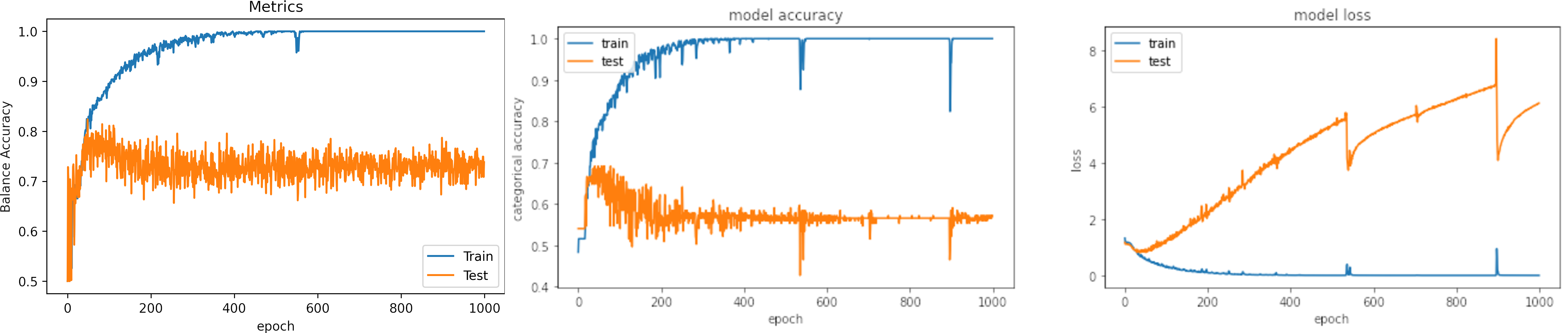
What can we observe on the plots?
- The model reaches training
accuracy = 100%andloss = 0.0011after 500 iterations. - It requires longer time that with a larger learning rate and the loss is bigger.
- Test loss increases.
- The result of testing varies in a small range.
- On two occasions, the model fell into the wrong minima and had an inadequate result.
- The results are:
loss: 6.303
Accuracy: 0.559
Balance Accuracy: 0.456
Learning rate OK, learning_rate = 1e-3
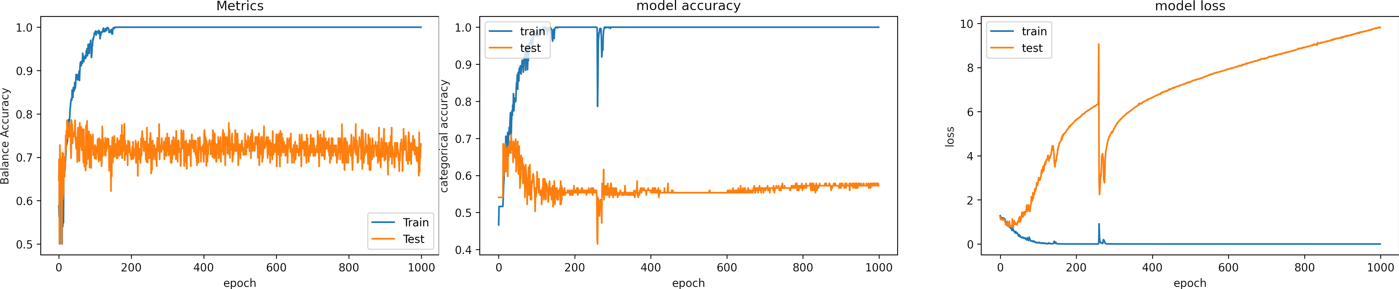
What can we observe on the plots?
- The model reaches training
accuracy = 100%andloss = 1e-6after 300 iterations. - It requires less time to converge, around 150 epochs.
- Test loss increases.
- In one occasions, the model fell into the wrong minima and had an inadequate result.
- The model learns for the training data, which means the learning rate is adequate.
- Around epoch 250, the model fell into the wrong minima and had an inadequate result; fortunately, it could escape.
- The results are:
loss: 9.819
Accuracy: 0.591
Balance Accuracy: 0.420
Learning rate scheduler
We can define a function that decreases a initial learning rate during the training process.
Exponential scheduler
This function keeps the initial learning rate for the first N epochs and decreases it exponentially.
We can fix the learning rate until EPOCH_N = 10, and Initial learning_rate = 0.01.
Our network already has a low loss at this value, and then we decrease the learning rate.
The exponent of "e" controls the rate of change.
def scheduler(epoch, lr):
    EPOCH_N = 10
    if epoch < EPOCH_N:
        return lr
    else:
        return lr * tf.math.exp(-0.01)
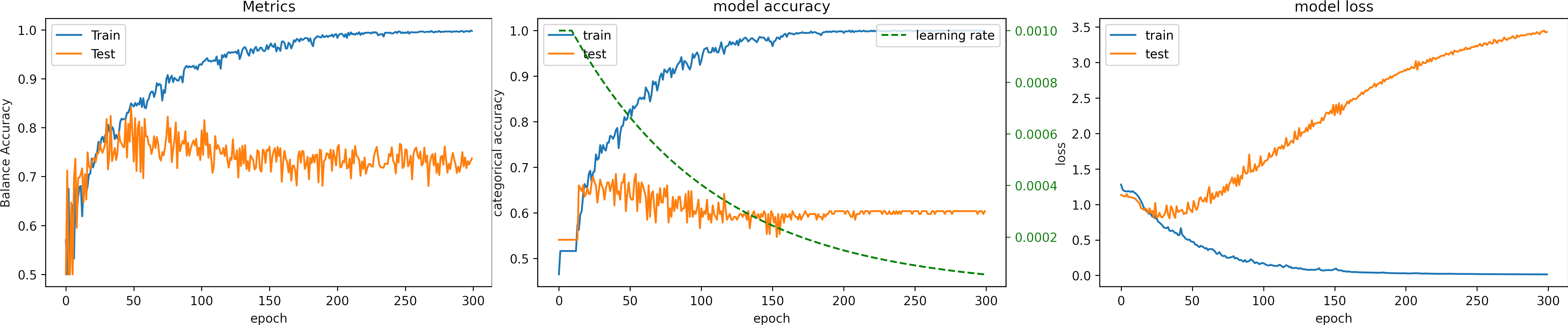
What can we observe on the plots?
- The model reaches a high accuracy after 200 epochs.
- The minimum loss is
loss=0.01, much higher than in previous experiments. - The fluctuations for testing accuracy and loss are reduced.
- We can observe how the learning rate decreases (green line).
- The fluctuations in testing accuracy and loss reduce when the learning rate decreases.
- The learning rate become too low that there are no variations soon after 200 epochs.
- A large LR at the beginning speeds up the training, and lowering the value prevents the learning from fluctuating.
- Testing loss increases, and testing accuracy does not improve.
- The final result for testing:
loss: 3.429
Accuracy: 0.578
Balance Accuracy: 0.419
Ladder scheduler
This function drops the learning rate, every epochs_drop epochs.
We can set the epochs_drop=20, drop_rate=0.9 and Initial learning_rate = 0.01.
The drop rate controls the rate of change.
def lr_step_decay(epoch, lr):
    drop_rate = 0.9
    epochs_drop = 20.0
    return initial_learning_rate * math.pow(drop_rate, math.floor(epoch/epochs_drop))
What can we observe on the plots?
- The model reaches a high accuracy before 150 epochs.
- The minimum loss is
loss 1e-4. - We can observe how the learning rate decreases (green line).
- The fluctuations in testing accuracy and loss reduce when the learning rate decreases.
- The learning rate decreases in steps, we can modify the function
lr_step_decayfor a faster or slower decay. - Testing loss increases, and testing accuracy does not improve.
- The final result for testing is better than in previous cases:
loss: 5.017
Accuracy: 0.572
Balance Accuracy: 0.389
New model definition
The results show very similar accuracy values for different learning rates.
Thus, the learning rate controls the training speed and ensures convergence but does not improve the result.
Therefore, we define a more complex model including pooling operations and Dropout layer.
:
def get_new_model_v2():
    model = tf.keras.Sequential([
            keras.Input(shape=(696, 1)),
            keras.layers.Conv1D(32, 5, padding="valid", use_bias=True, activation='relu'),
            keras.layers.MaxPooling1D(pool_size=2),
            keras.layers.Conv1D(64, 5, padding="valid", use_bias=True, activation='relu'),
            keras.layers.MaxPooling1D(pool_size=2),
            keras.layers.Conv1D(128, 5, padding="valid", use_bias=True, activation='relu'),
            keras.layers.MaxPooling1D(pool_size=2),
            keras.layers.Flatten(),
            keras.layers.Dense(256, activation='relu'),
            keras.layers.Dropout(.2),
            keras.layers.Dense(4, activation='softmax')
        ])
    return model
What can we observe on the plots?
- The model reaches a high accuracy in around 200 epochs.
- We can observe how the learning rate decreases (green line).
- There are high fluctuations in testing accuracy. Thus the result depends on the value obtained at a specific epoch.
- Dropout layer deactivates random neurons.
- The model does not overfit due to the Dropout layer.
- The minimum loss is
1e-4. - The final result for testing:
loss: 5.469
Accuracy: 0.679
Balance Accuracy: 0.456
Learning rate summary
| Learning rate | value | pros | cons | Epochs | Loss | Accuracy | Balance Accuracy |
|---|---|---|---|---|---|---|---|
| Large | 0.001 | Fast | May Diverge, large variations | 300 | 8.318 | 0.572 | 0.365 |
| Small | 1e-4 | Converge, low variations | Slow, it can fall into local minima | 500 | 6.136 | 0.559 | 0.456 |
| OK | 1e-3 | Converge | medium or fast speed | 200 | 9.819 | 0.591 | 0.420 |
| Exponential scheduler | 1e-3 to 1e-5 | Converge, smooth changes | Fast | 200 | 3.429 | 0.578 | 0.419 |
| Ladder scheduler | 1e-3 to 1e-4 | Converge, easier to define | Fast, changes by steps | 150 | 5.017 | 0.572 | 0.389 |
| New model | 1e-3 to 1e-4 | Converge, no overfit | slow | 300 | 5.469 | 0.679 | 0.456 |
2D Convolutional Neural Networks (CNNs) on Tensorflow
2D and 1D CNNs have similar hyperparameters and similar problems.
However, 2d models have an advantage. The pre-trained models can be used to speed up training.
This section seeks to resolve some frequent questions and avoid possible errors in 2D CNN in Tensorflow.
Here you will see fractions of code, the complete code can be found in a GitLab repository (Python Course).
It contains series of Jupyter notebooks that will help you understand the basics of python and Tensorflow.
The examples given do not only seek to solve a specific problem.
Many exercises are written so that the concepts can be generalized.
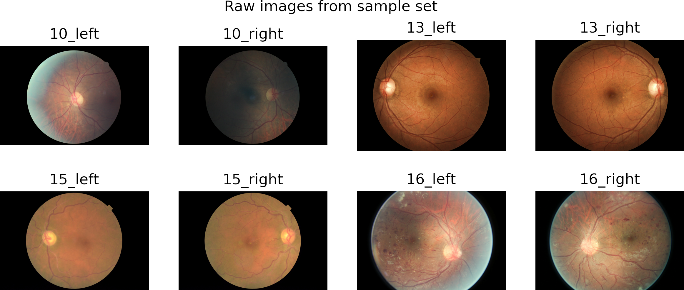
Download and load the data
We will use the Diabetic Retinopathy Detection challenge dataset.
It is a large set of high-resolution retina images.
Visit session3.2_get_data_from_the_internet
for more information about how to download datasets from kaggle.
The dataset is divided into training, validation, and testing so that no cross-validation is needed if we want to participate in the challenge.
| Split | Examples |
|---|---|
| Test | 42,670 |
| Train | 35,126 |
| Validation | 10,906 |
The dataset has four classes rated by a clinician. The presence of diabetic retinopathy is graded from 0 to 4 according to the following scale:
| Class | Severity level |
|---|---|
| 0 | No DR |
| 1 | Mild |
| 2 | Moderate |
| 3 | Severe |
| 4 | Proliferative DR |
As is typical in challengers, we do not have the test data values, so we are going to split the training set to test our models.
We first visualize the distribution of the classes.
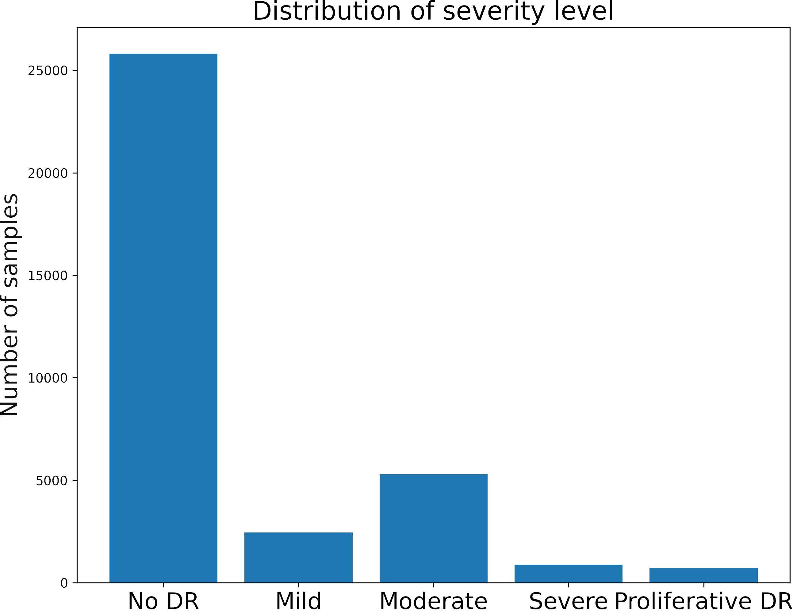
The dataset is highly unbalanced.
There are some alternatives to handle this type of problem. We will use only a part of the data of class 0 for training (5000 images).
We can not use global accuracy metrics. However, we can use sensitivity which gives us a metric regarding the classifications of each class.
During training, we evaluate our model on validation data every n epochs to speed up the training process.
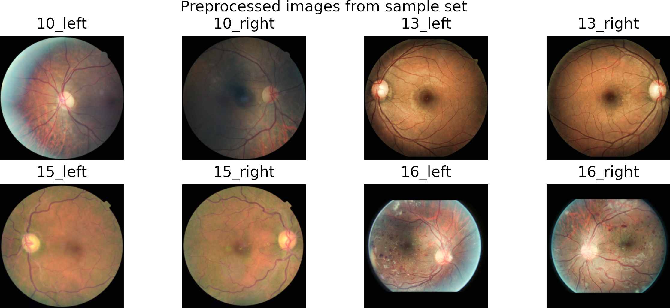
Prepare raw data
Follow this
Jupyter notebook to prepare the data.
In preprocessing, we crop the region of interest from the images. Then we resize it to a square image by padding the smaller dimension with zeros.
We use the Contrast Limited Adaptive Histogram (CLAHE) algorithm to enhance local contrast.
Finally, we save the images into folders corresponding to each class.
Model definition
The Jupyter notebook can be found here .
We define a simple model using a pretrained model (MobileNetV2).
We set the image size to 224,224,3.
The network freezes the base model parameters and uses the GlobalMaxPooling2D to generate a global feature that passes through three dense layers.
def get_pretrain_model(network='VGG16', nClass=2, img_width=32, img_height=32):
    """
    This function returns  a simple 2D CNN model.
    It use as base model a pretrain model
    network (string) : select an option 'VGG16', 'MobileNetV2', 'ResNet50' or'InceptionV3'
    nClass (int) : number of classes
    img_widht (int) : input image widht
    img_height (int) : input image height

    return a tensorflow model
    """
    # Define model
    if network=='VGG16':
        base_model = vgg16.VGG16(weights='imagenet',include_top=False, input_shape=(img_height, img_width,3))
    elif network =='MobileNetV2':
        base_model = mobilenet_v2.MobileNetV2(weights='imagenet',include_top=False, input_shape=(img_height, img_width, 3))
    elif network == 'ResNet50':
        base_model = resnet50.ResNet50(weights='imagenet',include_top=False, input_shape=(img_height, img_width, 3))
    elif network == 'InceptionV3':
        base_model = inception_v3.InceptionV3(weights='imagenet',include_top=False, input_shape=(img_height, img_width, 3))

    base_model.trainable = False
    x = base_model.output
    x = GlobalMaxPooling2D()(x)
    x = Dense(2048, activation='relu')(x)
    x = Dense(256, activation="relu" )(x)
    x = Dense(nClass, activation='softmax')(x)

    return Model(base_model.input, x)
Neither the network configuration nor the final classification is our primary interest in this practice. Our goal is to recognize when the learning rate is adequate or not.
Define a number of epochs
There is no rule to define the number of necessary epochs. Some conditions require more epochs:
- CNN with several layers to train.
- A small learning rate.
- A large dataset.
In this case, the network is extensive. However, the number of learnable parameters is small, and we do not require many epochs.
We set epochs = 1000 to check how the training parameters respond (loss and accuracy). Later we reduce this number.
Learning rate too Large, learning_rate = 0.01
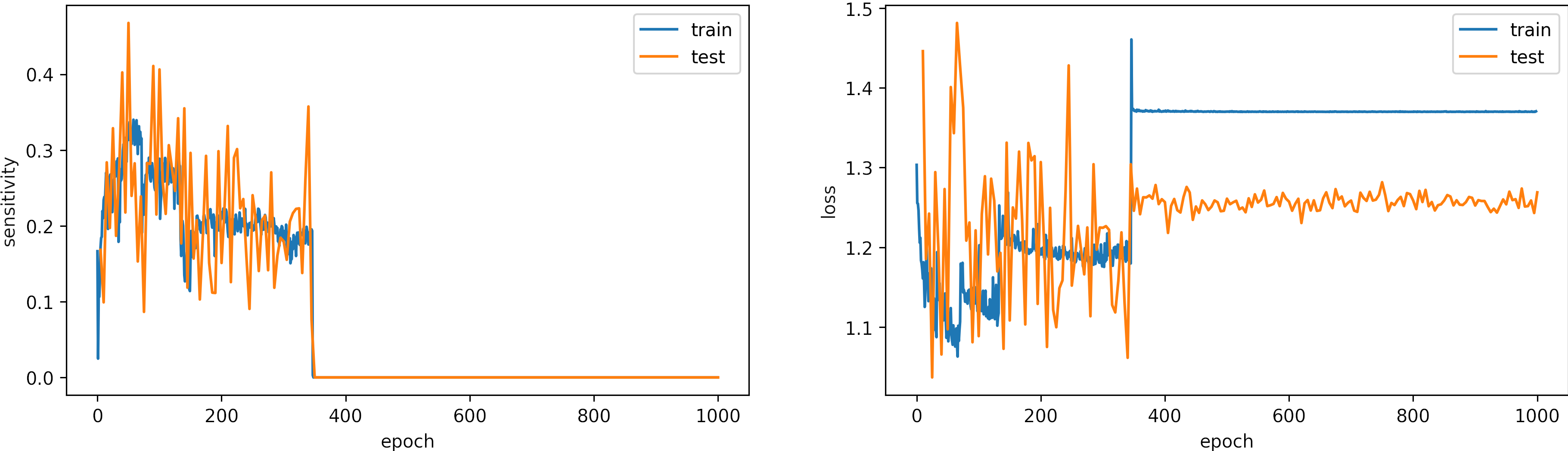
What can we observe on the plots?
- The model accuracy decreases over time, and the loss increases.
- The learning rate is too high, producing large fluctuations in the model accuracies and losses.
- Around the epoch 400, the model diverges.
- It is a better idea to set early stopping to avoid running unnecessary iterations
- The results:
loss: 1.269
Sensitivity: 0.0
Large learning rate, learning_rate = 0.001
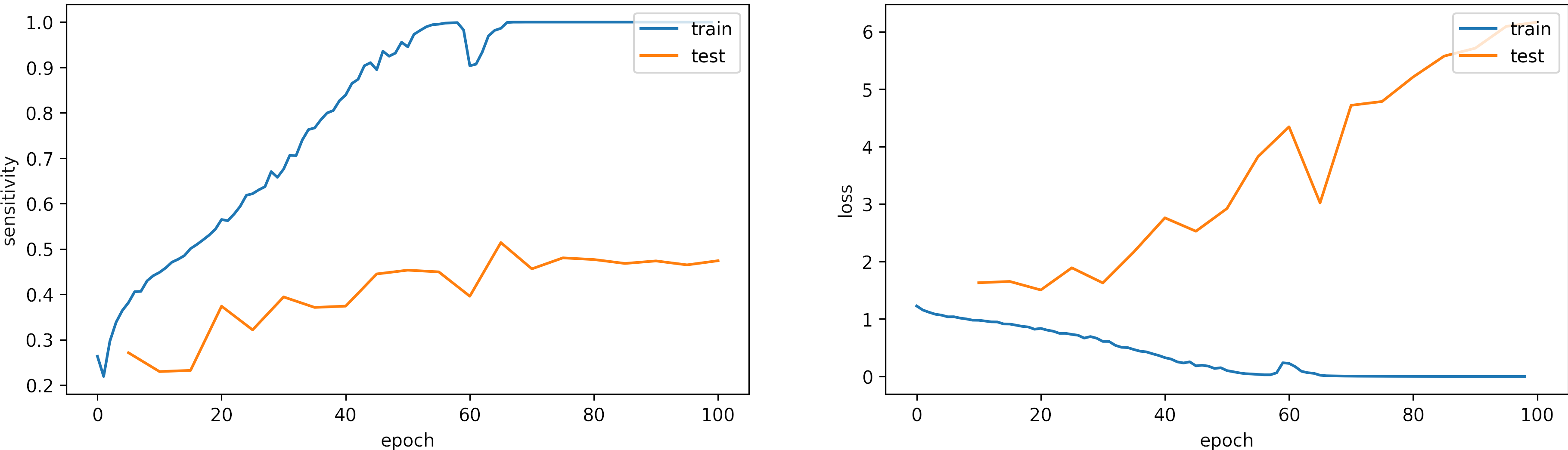
We set the epochs = 100.
What can we observe on the plots?
- The model reaches training
sensitivity = 100%andloss <= 0.03after 70 iterations. - The validation accuracy is low, however the learning rate is adequate.
- Early stopping is an alternative to selecting a fixed number of iterations because the model may be in a lower spike or recovering from it in a given iteration.
- For this configuration, from 70 to 100 epochs are enough.
- The results are:
loss: 6.166
sensitivity: 0.472 - We need to change the arquitecture or apply augmentation.
Learning rate small, learning_rate = 1e-5
We set the epochs = 200.
What can we observe on the plots?
- The model needs arround 150 epochs to reaches
sensititivy=1.0for training and low loss. - The testing accuracy increases but keeps constant. However, the test loss increases, which shows some overfitting.
- The fluctuations in the accuracy and loss are minor.
- For this configuration, 200 epochs are not enough, we will train the model with a larger learning rate, we expect to need less iteration to converge.
- The results are:
loss: 2.611
categorical_accuracy: 0.361
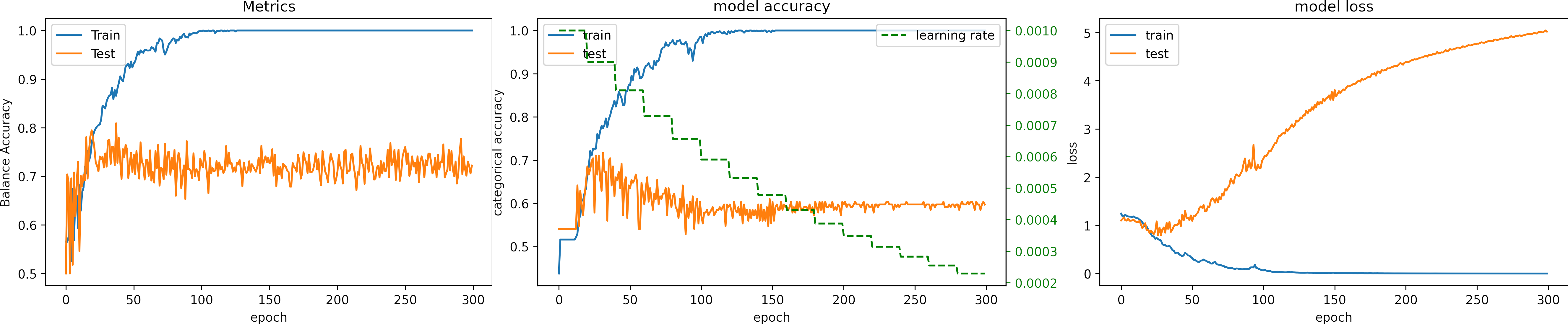
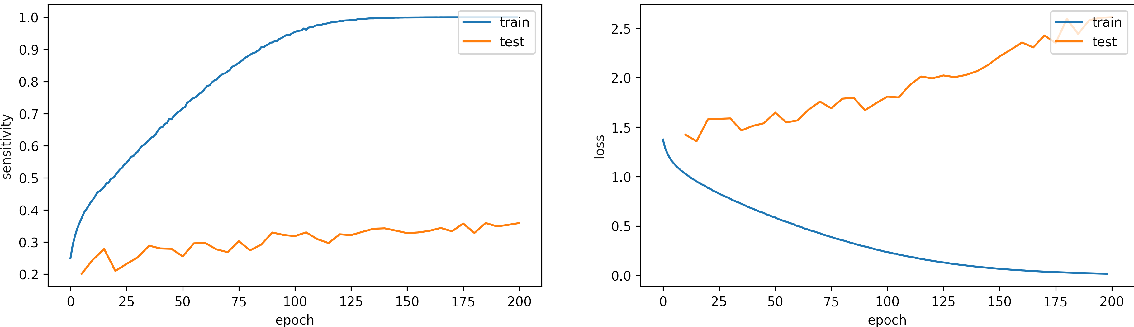
Learning rate OK, learning_rate = 1e-4
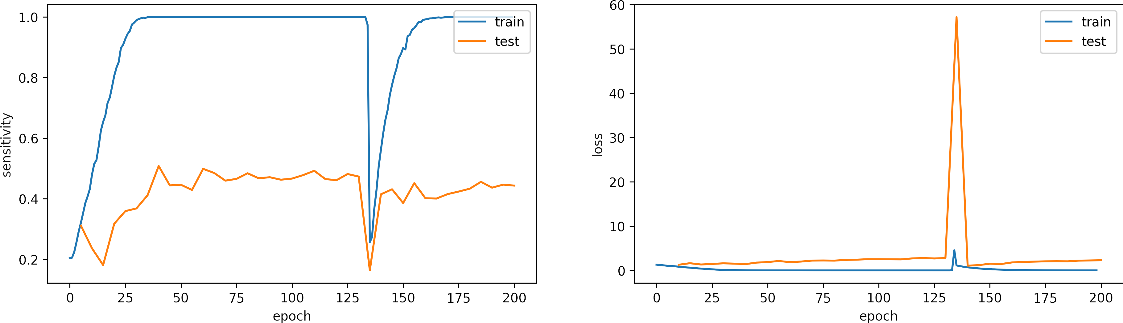
We set the epochs = 200.
What can we observe on the plots?
- The model reaches training
sensitivity = 100%andloss <= 0.03after 40 iterations. - The validation accuracy is low, however the learning rate is adequate.
- In epoch 136, the model was about to diverge but could be recovered.
- Early stopping is an alternative to selecting a fixed number of iterations because the model may be in a lower spike or recovering from it in a given iteration.
- For this configuration, from 50 to 100 epochs are enough. We expect to need less iteration with a slight larger learning rate.
- Thus, before execute cross-validation, it is ok check one fold.
- The results are:
loss: 2.294
sensitivity: 0.440 - We need to change the arquitecture or apply augmentation.
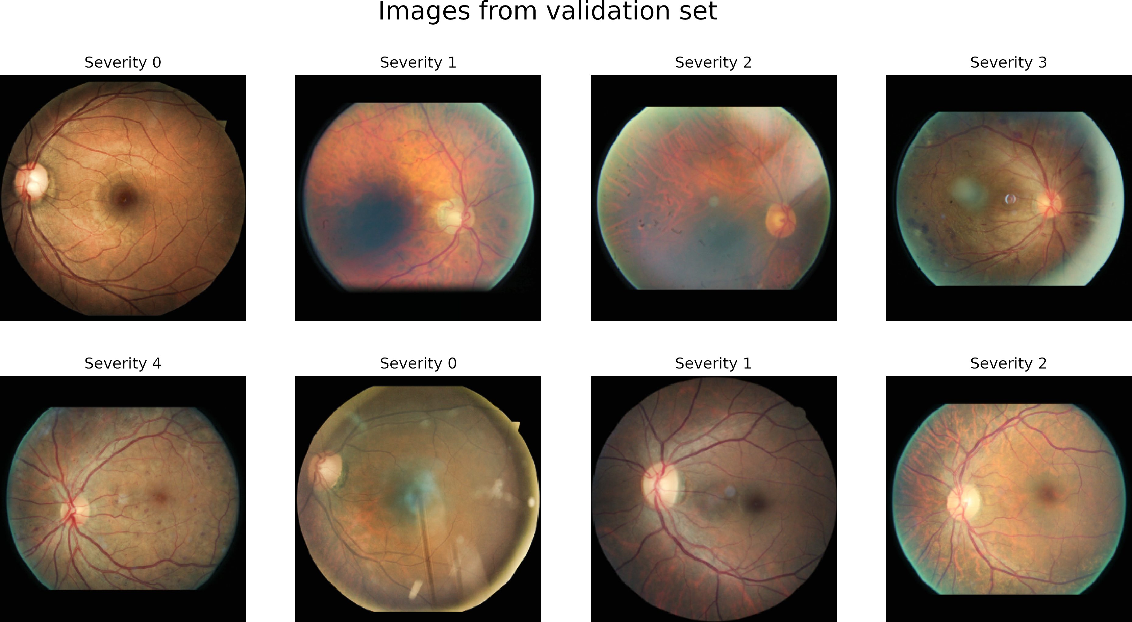
Data Augmentation
Data augmentation generates variations in the training data with physical consistency.
It allows the model to be more general and not only memorize the initial data.
We create a function that randomly rotates the image and central crop the image.
def rotate(x , labels):
    """Rotation augmentation

    Args:
        x: Image

    Returns:
        Augmented image
    """
    x = tf.cast(x, dtype=tf.float32)

    # Rotate random*369 degrees
    if np.random.rand(1)>.2:
        x = tf.image.convert_image_dtype(x, tf.float32)
        x = tfa.image.rotate(x, tf.image.convert_image_dtype(2*np.pi*np.random.rand(1), tf.float32))
        x = tf.convert_to_tensor(x, dtype=tf.float32)
        x = tf.image.resize(x, [IMG_HEIGHT, IMG_WIDTH])
        x = tf.cast(x, dtype=tf.float32)

    return x, labels

The figure shows some preprocessed images on the top and a rotated version on the bottom.
The two most common alternatives in data augmentation are:
- Create a new fixed data set containing the original and augmented data, makes the dataset larger.
- Increase data during training, same size dataset. However, it will require more epochs to converge.
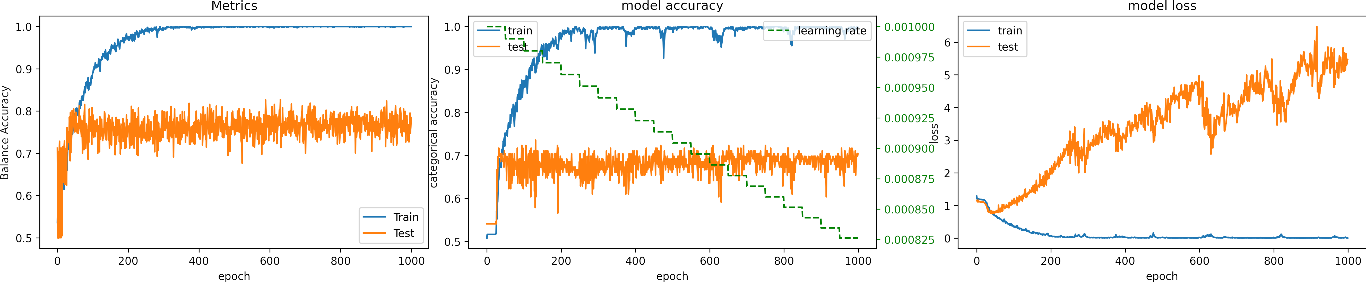
We select the second approach, and we set the number of epochs to 500, we set the learning_rate = 1e-4.

What can we observe on the plots?
- The model reaches a high accuracy.
- It requieres 500 epochs to converge.
- Testing loss increases because the model overfit.
- The final accuracy for testing is better than in previous cases:
loss: 5.483
categorical_accuracy: 0.496
New model + Data Augmentation
We include a SeparableConv2D and Dropout layers after the Dense layers.
The dropout layer randomly sets units to 0 with a frequency of rate (in our net 0.2) at each step during training time, which helps prevent overfitting.
We augmented the data with the rotation function described before.
Code.
def get_pretrain_model_v2(network='VGG16', nClass=2, img_width=32, img_height=32):
  """
  This function returns a simple 2D CNN model.
  It use as base model a pretrained model
  network (string) : select an option 'VGG16', 'MobileNetV2', 'ResNet50' or'InceptionV3'
  nClass (int) : number of classes
  img_widht (int) : input image widht
  img_height (int) : input image height

  return a tensorflow model
  """

  # Select pretrained model
  if network=='VGG16':
      base_model = vgg16.VGG16(weights='imagenet',include_top=False, input_shape=(img_height, img_width,3))
  elif network =='MobileNetV2':
      base_model = mobilenet_v2.MobileNetV2(weights='imagenet',include_top=False, input_shape=(img_height, img_width, 3))
  elif network == 'ResNet50':
      base_model = resnet50.ResNet50(weights='imagenet',include_top=False, input_shape=(img_height, img_width, 3))
  elif network == 'InceptionV3':
      base_model = inception_v3.InceptionV3(weights='imagenet',include_top=False, input_shape=(img_height, img_width, 3))

  # Let's take a look to see how many layers are in the base model
  print("Number of layers in the base model: ", len(base_model.layers))

  base_model.trainable = False

  x = base_model.output
  x = tf.keras.layers.SeparableConv2D(1280, 3, padding="valid", use_bias=True, activation='relu')(x)
  x = GlobalMaxPooling2D()(x)
  x = Dense(1024, activation='relu')(x)
  x = keras.layers.Dropout(.2)(x)
  x = Dense(256, activation="relu" )(x)
  x = keras.layers.Dropout(.2)(x)
  x = Dense(nClass, activation='softmax')(x)
  pretrain_model = Model(base_model.input, x)

  return pretrain_model
We set the number of epochs to 100, we set the learning_rate = 1e-4.
The Visualization App 3 shows Relevance map (R-map) that indicates which pixels are relevant for predicting a given class for this model.
Please visit App 3.

What can we observe on the plots?
- The model reaches a high accuracy after 30 epochs.
- The model converges fast, and the test accuracy remains constant.
- Testing loss increases because the model overfit.
- The final accuracy and loss for testing are better than in previous cases:
loss: 2.554
categorical_accuracy: 0.554
Learning rate summary
| Learning rate | value | pros | cons | Epochs | Loss | Accuracy |
|---|---|---|---|---|---|---|
| Too Large | 0.01 | -- | Diverge, large variations | +300 | 1.269 | 0.000 |
| Large | 0.001 | Fast | Medium variations | 70 | 6.166 | 0.472 |
| Small | 1e-5 | Converge, low variations | Slow | 150 | 2.611 | 0.361 |
| OK | 1e-4 | Converge, fast | - | 40 | 2.294 | 0.440 |
| Data augmentation | 1e-4 | Converge, no overfit | slow | 50 | 5.483 | 0.496 |
| New model+Data augmentation | 1e-4 | Converge, fast | - | 30 | 2.554 | 0.554 |